Hash tables are fundamental data structures in computer science, celebrated for their average O(1) time complexity for insertion, deletion, and lookup operations. However, one inherent challenge they face is hash collisions—a scenario where two distinct keys produce the same hash value. In this blog post, we’ll explore what hash collisions are, why they matter, and the most effective strategies to resolve them.
Understanding Hash Collisions
A hash function converts an input (key) into a fixed-size integer (hash code), which maps to an index in an array (the hash table). Due to the pigeonhole principle—where there are more possible keys than available indices—collisions are inevitable. For example, if a hash table has 100 slots, two different keys will eventually hash to the same index.
While collisions can’t be eliminated entirely, managing them efficiently is critical. Poor collision resolution leads to degraded performance, potentially worsening to O(n) time complexity in the worst case.
Common Strategies to Resolve Hash Collisions
Let’s dive into the most widely used techniques to handle hash collisions, along with their pros, cons, and use cases.
1. Open Addressing
Open addressing (or closed hashing) resolves collisions by finding an alternative empty slot in the hash table when the original index is occupied. It relies on probing—systematically checking subsequent slots until an empty one is found.
Types of Probing:
- Linear Probing: Check the next slot (index + 1, index + 2, etc.) sequentially. Simple to implement but suffers from clustering—consecutive occupied slots that increase probe length.
- Quadratic Probing: Use a quadratic function (e.g., index + 1², index + 2²) to skip slots. Reduces clustering but may not explore all slots if the table size is poorly chosen.
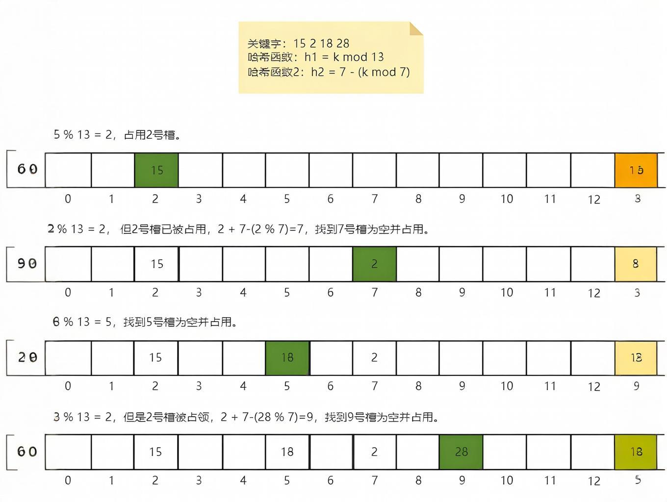
- Double Hashing: Apply a second hash function to determine the step size for probing. Eliminates clustering but requires designing a robust secondary hash function.
Pros:
- Uses a single array, making it memory efficient.
- Faster access due to better cache locality (data is stored contiguously).
Cons:
- Performance degrades with high load factors (typically limited to 0.7).
- Deletion is complex—requires marking slots as “tombstones” to avoid breaking probe sequences.
Use Case:
Ideal for small, fixed-size datasets where memory efficiency is critical (e.g., embedded systems).
2. Separate Chaining
Separate chaining (or open hashing) resolves collisions by storing all keys that hash to the same index in a linked list (or another data structure). Each slot in the hash table points to the head of a chain.
How It Works:
- When a collision occurs, the new key is appended to the linked list at the collided index.
- Lookups traverse the linked list to find the target key.
Pros:
- Simple to implement and handle deletions.
- Performance degrades gracefully with high load factors.
- No clustering issues.
Cons:
- Extra memory overhead for storing pointers (or references) in linked lists.
- Poor cache performance due to scattered memory access.
Optimization:
Modern implementations often replace linked lists with balanced trees (e.g., Java’s HashMap uses red-black trees for large chains) to reduce lookup time from O(n) to O(log n).
Use Case:
Widely used in general-purpose hash tables (e.g., Python’s dict, JavaScript’s Object) due to its flexibility.
3. Coalesced Hashing
Coalesced hashing combines elements of open addressing and separate chaining. Collided keys are stored in empty slots, but each slot maintains a pointer to the next key in its chain.
Pros:
- Reduces memory overhead compared to separate chaining.
- Avoids clustering better than linear probing.
Cons:
- More complex to implement than other methods.
- Probe sequences can still become long in large tables.
4. Perfect Hashing
Perfect hashing uses a two-level hash table to guarantee O(1) lookups with no collisions. The first level maps keys to a secondary hash table, which is sized to avoid collisions for its subset of keys.
Pros:
- No collisions, ensuring optimal performance.
Cons:
- Requires preprocessing to design hash functions, making it unsuitable for dynamic datasets.
- High memory usage for secondary tables.
Use Case:
Static datasets with known keys (e.g., dictionary lookups in compilers).
Choosing the Right Strategy
The choice of collision resolution depends on your use case:
- Separate Chaining: Best for dynamic datasets with variable sizes.
- Open Addressing: Preferable for memory-constrained environments with low load factors.
- Perfect Hashing: Ideal for static datasets requiring guaranteed O(1) performance.
Additionally, hash function design plays a critical role. A good hash function minimizes collisions by distributing keys uniformly across the table. Common examples include the Jenkins hash, MurmurHash, and SHA-1 (for cryptographic applications).
Conclusion
Hash collisions are unavoidable, but with the right resolution strategy, their impact can be mitigated. Whether you opt for separate chaining’s simplicity, open addressing’s memory efficiency, or perfect hashing’s guaranteed performance, understanding these techniques is key to building efficient hash tables.
By balancing hash function quality, load factor, and collision resolution, you can ensure your hash table delivers the near-constant time complexity it’s known for.